Seven pivot-table practices that compound in FP&A

Pivot tables move from convenience tool to operating system once seven practices are in place. Each one is small. Together they cut hours out of the close and kill a class of silent reporting errors. The workbook below has the practice dataset and the reference output for every technique.

Range-bound pivots silently miss new rows. A pivot anchored to A1:G500 does not include the November paste into rows 501–540. The report refreshes, the chart updates, and the variance pack is wrong.

Format the source as an Excel Table (Ctrl+T) and rename it (tblSales). Build every pivot against the Table name. New rows flow through on refresh; structured references read cleanly:

=SUMIFS(tblSales[Revenue], tblSales[Region], "West")

Every other practice in this memo assumes the pivot is Table-backed.

Right-click any value cell → Show Values As. Excel offers eleven transforms of the underlying aggregate. Five carry the load:

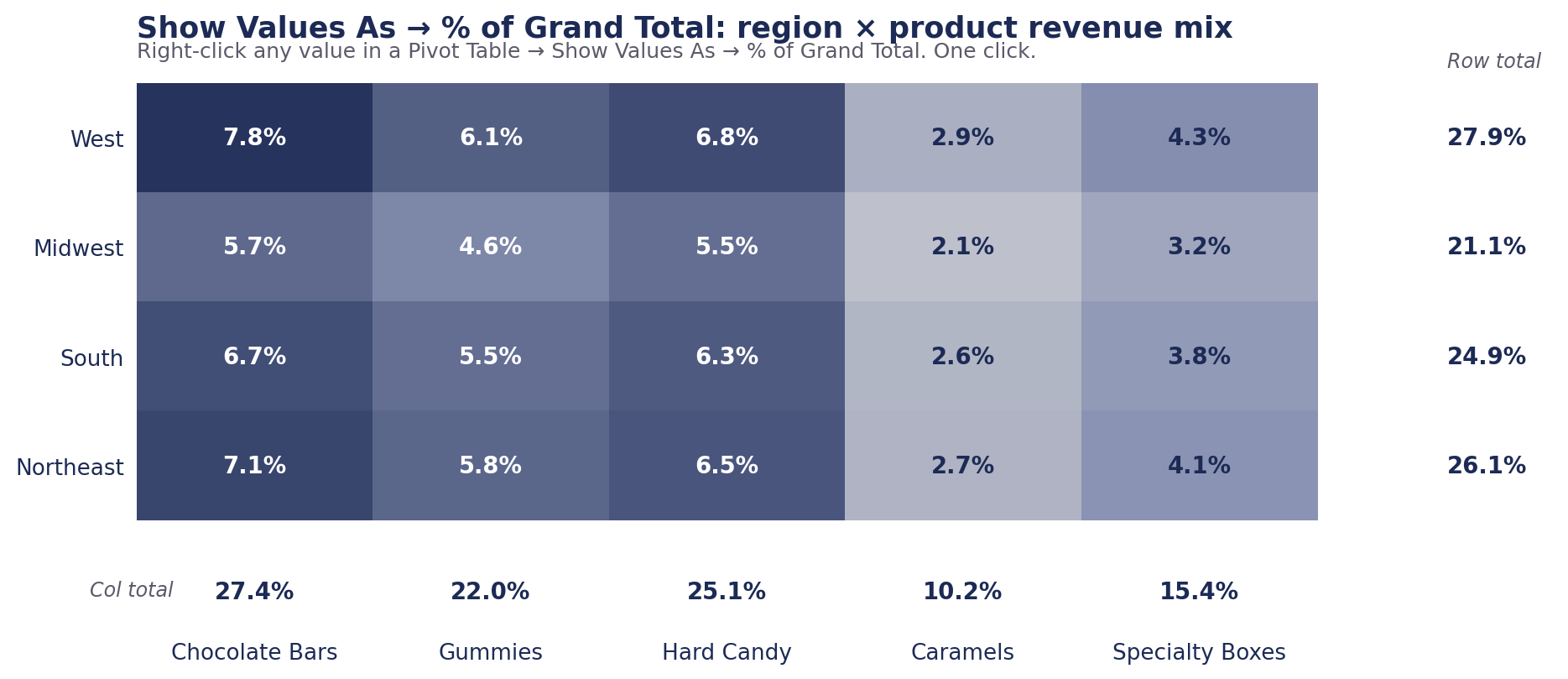
• % of Grand Total. Each cell as its share of the whole. Mix analysis, customer concentration.
• % of Parent Row Total. Mix within each group, computed separately per group.
• Running Total In. Cumulative across the chosen field. YTD by month without a SUMIFS chain.
• Difference From (previous). Month-over-month dollar variance.
• % Difference From (previous). Month-over-month growth rate.

Gross margin computed as a source column and then averaged in the pivot returns the wrong number. The average weights every row equally; a $30 line counts as much as a $500,000 line.

Compute the ratio on aggregates. Add a Calculated Field (PivotTable Analyze → Fields, Items & Sets → Calculated Field):

=('Revenue' - 'COGS') / 'Revenue'

The pivot now reports margin weighted correctly at every level.

When clicked from another cell, a pivot cell returns a verbose formula:

=GETPIVOTDATA("Revenue", $A$3, "Region", "West", "Product", "Specialty Boxes")

The verbosity is the feature. References resolve by field name and value, not cell address. The pivot can resort, expand, or filter without breaking the board-deck formula.

Pattern: one flat pivot on a hidden tab (Pivot_Engine); the executive layout on a separate visible tab; every value cell a GETPIVOTDATA reference. Drift between numbers and report goes to zero.

Right-click a slicer → Report Connections → tick the other pivots. One click drives the whole dashboard.

Constraint: slicers connect only to pivots that share a pivot cache. Pivots built from one Excel Table via the default insert flow share one. Mixing source Tables or connection routes splits the cache.

About to write VLOOKUP on the source data? Stop. Add the lookup as a separate Table and tick “Add this data to the Data Model” at pivot-create time. Three capabilities follow:

• Relationships between Tables. No more VLOOKUP-then-pivot.
• Distinct Count. Unimaginable in a classic pivot; built in here.
• DAX measures. Filter inside the calculation; same language Power BI uses.

The trade: harder to teach, harder to audit. The signal it earns its complexity is real cross-Table joins, not a single flat dataset.

Microsoft shipped native array-formula equivalents in 2024. Same output as a pivot, no refresh, no pivot cache:

=GROUPBY(tblSales[[Region]:[Product]], tblSales[Revenue], SUM, 3, 0)

=PIVOTBY(tblSales[Region], tblSales[Product], tblSales[Revenue], SUM, 3, 0, 3, 0)

Use them where the report is fixed and downstream formulas need to update automatically. Use pivots where the analyst will drag fields and drill down. Excel 365 with the 2024+ build only.

Four tabs. Source data is 1,440 rows of synthetic candy-shop sales as Table tblSales. Tab 03 is the reference: every section above as a live array formula spilling off the source — PIVOTBY, SUMIFS, SCAN, LET. Add a row to tblSales and every output recomputes.